To prevent ore from wearing out grinding mill drums, replaceable liners are inserted. ABB and Bern University of Applied Science have developed a liner wear monitoring system based on accelerometers and machine learning that identifies the best time to change the liner and thus reduce downtime costs.
Venkat Nadipuram ABB Process Industries, Mining, Aluminium and Cement Baden-Daettwil, Switzerland, venkat.nadipuram@ch.abb.com; Marco Jordi, Prof. Dr. Axel Fuerst Bern University of Applied Science Institute for Intelligent Industrial Systems, I3S, Burgdorf, Switzerland
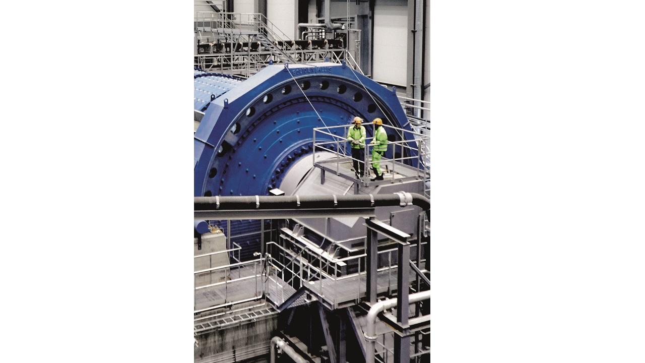
In large mines, ore is milled onsite to extract valuable minerals. The grinding mills that perform this extraction consist of a large drum in which the ore itself, and sometimes added steel balls too, carry out the physical grinding process. As the drum rotates, the ore/balls are lifted up the side of the drum’s interior by vanes to the cascading angle, where they fall off and crash to the bottom, reducing the ore.
As drum diameters can be as large as 10 m, the drum is an expensive piece of kit. To prevent damage to the drum, metal or rubber liners are inserted. The costs of liner replacement are high due to mill downtime and replacement parts so it is economical to change the liner as late as possible, but also at a time that minimizes productivity loss. To achieve this goal, it is important that the actual liner wear is known. The wear can be measured from inside the mill but this requires a costly production stop. A method to detect wear during operation is therefore desirable →1.
Vibration monitoring
As the ore hits the liner, vibrations arise. These vibrations and their transfer function have been shown to change with liner thickness and this effect underlies a promising method to measure wear. Accordingly, ABB and The Institute for Intelligent Industrial Systems (I3S) at Bern University of Applied Science, conducted harmonic response and transient simulations to investigate this behavior. The results showed clearly that the amplitude of the acceleration signal from a worn liner is higher than that from a new liner.
To verify these findings and because access to a real ore mill is difficult, a scale model of a mill was built →2. With this prototype, many experimental measurements with different liner thicknesses were performed by ABB and I3S. All measurement data was analyzed with deep neural networks and classified with a high accuracy in the correct wear classes.

02a Scale model of an autogenous mill for experimental measurements in the lab. The model consists of a steel drum, driven by a toothed belt connected to a small electrical motor. The drum interior is covered with an interchangeable rubber layer to simulate the liner. 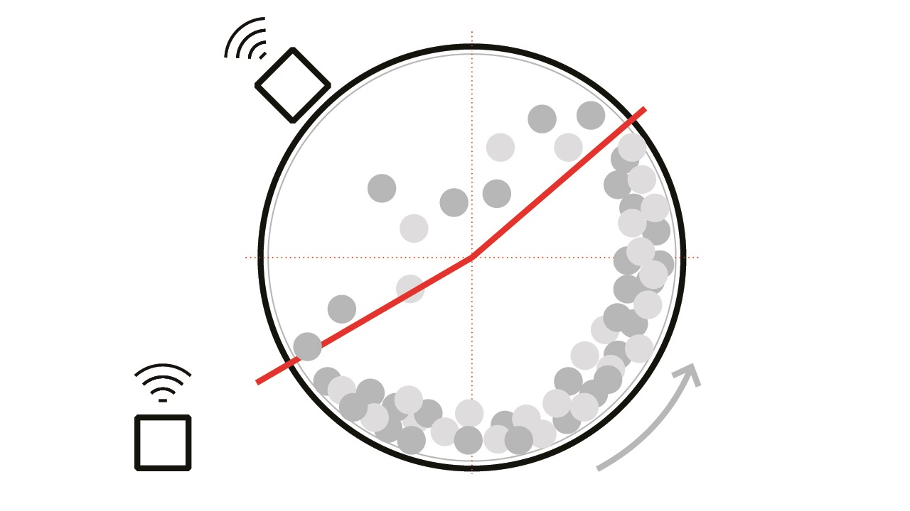
2b Function sketch of scale model with toe and shoulder angle and WLAN acceleration sensor. The sensor is placed on the outer surface of the drum to measure the vibration. The acceleration signal is the dependent variable; liner thickness and mill load are independent variables; and revolution speed, temperature, stone size and stone quality are controlled variables. Different measurements with 2 to 17 mm liner thickness and from 1 to 4 kg mill load was made. For each condition, at least two acceleration measurements of 2 min with a sampling frequency at 970 Hz were made.
02 Scale model
To transfer this process from the lab to a real mill environment, measurements were made at a real ore mill. With this data, I3S and ABB developed a prototype that allowed the liner condition and process parameters of a mill to be measured during operation.
Simulations
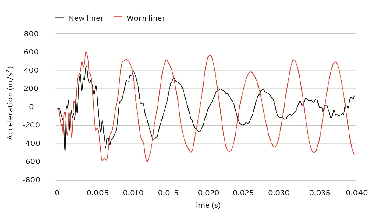
Harmonic response and transient finite element method (FEM) simulation in ANSYS [1] of new and worn-out liner models reinforced the idea that there is a measurable difference in the liner acceleration signal caused by ore impact at the drum wall between a new and a worn-out liner. For example, the frequencies from a worn liner are higher than those from a new liner. In effect, as the rubber wears, the damping properties decline. The main measurable differences in the simulations are in the amplitudes →3. This correlates to the theory that a thin rubber layer gives rise to a stronger impact, resulting in higher excitation forces.
Liner wear
The measurement of the liner thickness was made indirectly by acceleration sensors at the outer surface of the scale model drum.
The raw signal from these sensors was processed to extract features that can be used by a deep neural network to recognize patterns. The ”patternnet” (ie, pattern recognition network) used includes one input layer, three hidden layers each with 500 neurons and an output layer to classify the liner thickness.
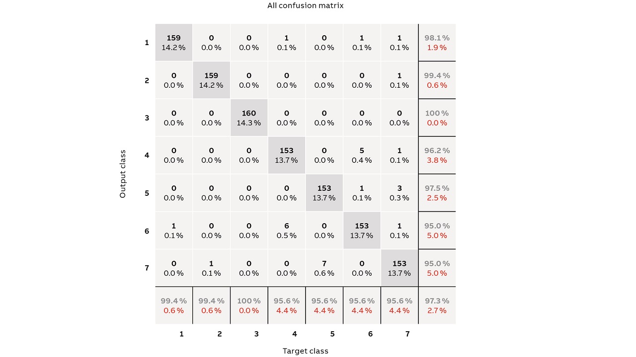
This configuration was used to classify the data from the scale model as well as from the field tests. In the laboratory, seven different liner conditions on the scale model were simulated. Liner thicknesses from 2 up to 17 mm and different loads reflect these conditions. The goal was to classify the preprocessed raw signal in one of the corresponding seven classes. The results showed a very high accuracy (close to 98 percent) for the scale model measurements. This means that only 2 percent of all the measurement datasets were classified falsely. This reflects the results from the training (70 percent) and the test (30 percent) dataset. →4 shows the confusion matrix of classification. Furthermore, data that is not correctly classified appears near to the matrix diagonal, which means the classification error is small.
The results from the field test measurements also showed a good accuracy. It was to be expected that the accuracy would be significantly lower here because of environmental effects but with an adapted deep neural network based on Tensorflow [2] a relatively high accuracy of 82.9 percent was achieved. The goal is to improve accuracy further with more data.
Toe and shoulder angles
To determine the cascading angle in the ore mill, the acceleration signal data from one turn of the real mill was used. In →5, the acceleration signal from one rotation is visible. In the impact zone, where stones hit the liner, high amplitudes are visible. Also, in the region of the shoulder angle, where the stones leave the liner, signal changes are visible. These arise because, in the area of the shoulder angle, the ore pieces lie loosely on top of each other. The gravity vector is shifting in relation to the position of the ore and the ore starts to leave the ore bed by sliding towards the center of the ore bed, creating vibrations at the mill shell.
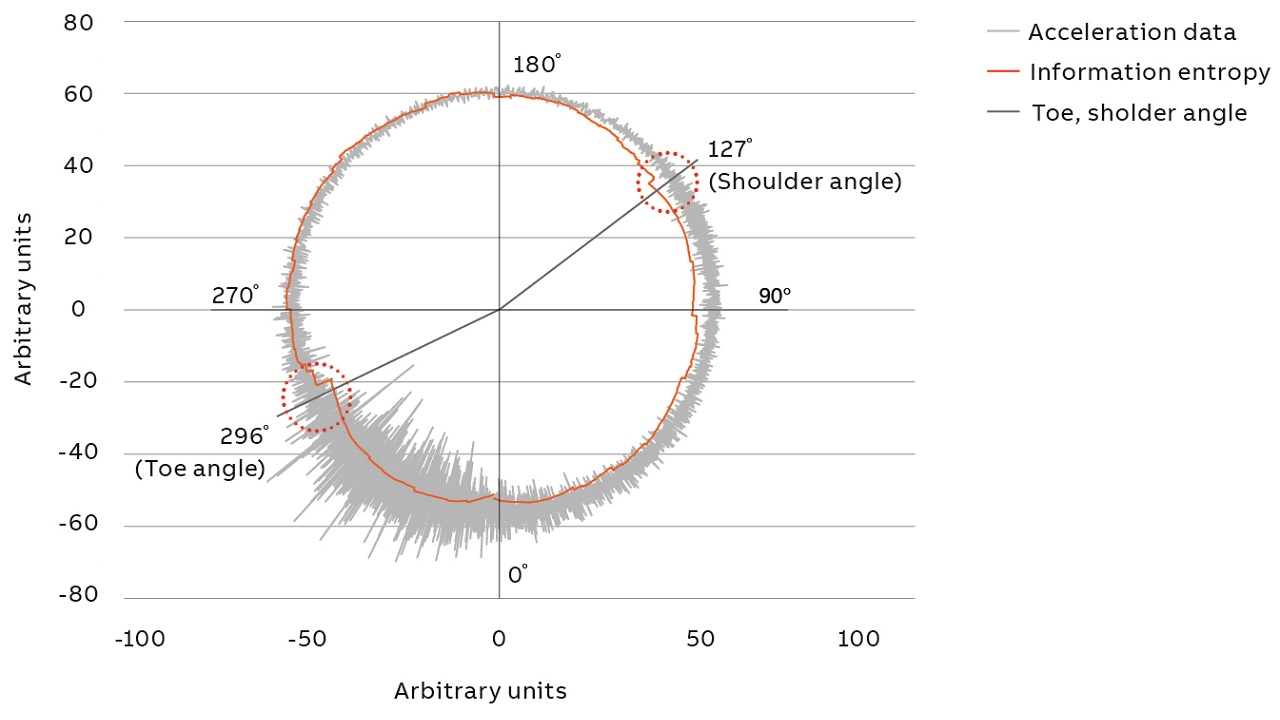
To find the toe and shoulder angle, the information entropy of the signal is calculated. The entropy of the signal (over a certain moving window) represents the amount of information contained in the signal [3]. In other words, the more random and unpredictable the acceleration signal due to the impacts is, the greater its entropy will be. Thanks to this calculation, changes in the acceleration signal and thereby the toe and shoulder angle can be detected. An important parameter is the window length of the calculated index. For this data, a window length of 1,180 samples shows good results.
Field tests
To verify the mathematical models, field tests were carried out. The sensitive sensor equipment was protected from the harsh and dirty mill environment by a robust metal enclosure. The equipment includes a battery, timer, several acceleration sensor drivers, an analogue-to-digital converter and a data acquisition device. The acceleration sensors themselves were mounted with magnets directly on the mill drum and their cables led back to the box. The enclosure was mounted on a fully operational mill and left to collect data for several weeks.
Data analysis with machine-learning techniques
The raw vibration signal is very noisy due to the many impacts recorded when the mill is rotating and it is difficult to distinguish the various liner conditions. Therefore, raw data preprocessing is necessary. Only with a standardized data basis it is possible to apply machine learning algorithms. Over many iterations, the best classification model was sought.
Preprocessing the data
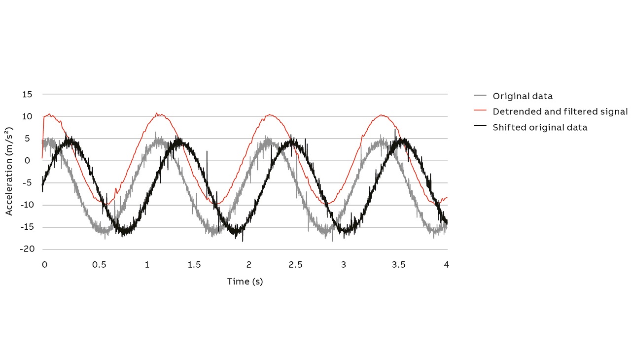
Because the measurement starting points are not the same every time, there are differences between the datasets. But for a proper evaluation it is necessary to have a uniform data basis. For this reason, a phase detector was included in the setup. The original signal was filtered through a low-pass filter (2 Hz cut-off frequency) and then a curve fitting and a detrending was applied. It was possible to determine the phase in the detrended and filtered data. This phase was then used to shift the original data so that all data sets have the same starting point →6.
After the phase shifter, the data from the 2 min measurements made was divided into slices representing one drum revolution. Additionally, the slices were resampled into 1,024 samples. This raw data preprocessing ensured a consistent data basis for the machine-learning algorithm.
Feature extraction
Machine-learning algorithms try to map a set of features to the correct target values. The right choice of these features is thus very important. Different features were tested, eg, wavelets, entropy and Fourier analysis. The best result was achieved with a combination of statistical values, the raw acceleration data and the FFT (fast Fourier transform) of each slice. All these features were combined into a table with the corresponding target value. This table is used as input matrix for the neural network.
Building a neural network for pattern recognition
To classify the data, different machine-learning methods such as support vector machines, decision trees or neural networks were tested. The best results were achieved with neural networks. A neural network should recognize patterns in each signal. These patterns help to classify the signal into a target class. Classes were built for all the measurements derived from the different mill load and liner thickness test runs.
After the definition of the classes, the input and output matrices for the neural network were constructed. The input matrix includes the feature table described above and the output matrix defines the correct target class for each feature set. Then a neural net [4] with three hidden layers each with 500 neurons and an output layer, for classification, was created →7.
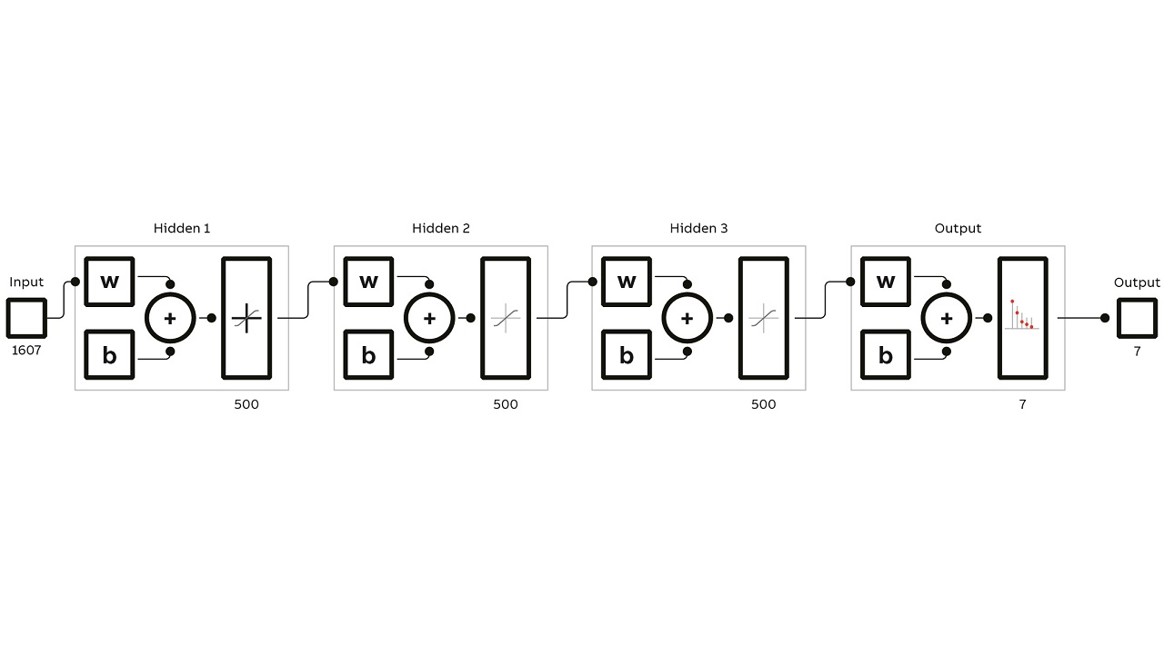
Of the data set, 70 percent was used for training the neural net, 15 percent for validation and 15 percent for testing the neural net. The network training employed a “scaled conjugate gradient backpropagation” – effectively a method that updates critical model parameters (neuron weights and bias) on the way through in an iterative fashion. Finally, a fine tuning of the network hyperparameters (ie, impactful parameters not tuned in the core model) that delivered an optimal neural network setting and enabled the liner condition to be determined reliably.
Liner monitoring for increased productivity and reduced costs
The hypothesis that the acceleration signal changes significantly with liner thickness was confirmed with simulations, and measurements on the scale model and on a real mill. The monitoring system developed by I3S and ABB shows how acceleration sensors and machine learning techniques can then be used to measure the condition and process parameters of a mill during operation. Thanks to the system, it will be possible to replace liners depending on their condition, which reduces downtime and costs while saving resources. This new monitoring system will help mill operators increase productivity and plan maintenance.
References
[1] ANSYS, Academic Research Mechanical, Release 18.1, ANSYS, Inc.
[2] M. Abadi et al., “TensorFlow: Large-Scale Machine Learning on Heterogeneous Systems,” preliminary white paper, Google, November 2015. Available: download.tensorflow.org/paper/whitepaper2015.pdf
[3] S. Vajapeyam, “Understanding Shannon’s Entropy metric for Information,” arxiv.org, March 2014. Available: arxiv.org/ftp/arxiv/papers/1405/1405.2061.pdf
[4] MATLAB, Neural Network Toolbox 2016a, The MathWorks, Inc., Natick, Massachusetts, United States.